Projecting 10 Year Portfolio Returns

Answering the following questions requires a view on future stock and bond portfolio returns:

• “How much can an endowment disburse and maintain its value?”
• “How much do I need to save for retirement?”
• “What is the likelihood of doubling my account in 5 years? 10 years?”

It is very difficult to predict market returns in the short term. However, most financial professionals and academicians believe that there is a rational approach to predicting portfolio returns over longer horizons as a basis for answering the important questions posed above.

Historically, equities have outperformed fixed income investments over time, but with much greater volatility in the returns achieved during each period. For an investor with an infinite or near infinite investment horizon, interim variability does not pose a challenge (other than emotional) as the equity market undergoes its normal ups and downs. For other investors, those with horizons of 5, 10, or even 30 years, the variability of returns can have a significant impact on the actual results achieved.

How does one plan for the future with equity returns, even over a 30-year period, being uncertain? It takes a solid understanding of both risk and return.

I. Risk

To understand the risks in the markets, we use Monte Carlo simulations. This is a modeling technique that was invented at the Los Alamos National Laboratory in the 1940’s and provides us with a probability distribution of returns. For example, Monte Carlo simulation provides an answer to the question, “Over a 10-year period, what is the probability that a client with a diversified portfolio of 64% stocks/36% fixed income will achieve an annualized return of at least 7%?”

We employ Modern Portfolio Theory to capture the risks in investing. Specifically, we use standard deviation and correlation to estimate the risks in the markets. Standard deviation is a measure of the degree to which returns of an asset vary from period to period, with a higher standard deviation indicating a higher degree of risk. Historically, stocks have had much higher standard deviations, or variability of returns, than fixed income. Correlation is the extent to which one asset moves in a linear relationship to another asset. A correlation of 1.0 indicates that two assets exhibit a 1:1 linear relationship in returns. Thus, if one asset increases 10% in value, the other asset would be expected to increase by the same percentage. A correlation of -1.0 indicates that two assets exhibit a 1:1 linear relationship, but in opposite directions. Thus, if one asset increases 10% in value, the other asset would be expected to decrease by the same percentage. A portfolio of assets having correlations of less than 1.0 has lower volatility than that of the individual assets, which is the cornerstone behind the rationale for diversification.

Standard deviation and correlation can be estimated based on history. We believe that 15 years of history is appropriate as it is a period long enough to smooth out anomalies yet short enough to reflect more recent market conditions on the assumption that recent experience is a better predictor of future events.

We apply standard deviation and correlation in the following multi-step manner for a portfolio’s equities.

• First, we obtain the standard deviation and correlation of indices that are representative of the assets within a client’s portfolios. For example, we use the Russell 2000 index as representative of U.S. small cap stocks within the portfolio and the Russell 2000 Value index as representative of U.S. small cap stocks having a high book-to-market value.
• Second, for the representative indices as well as the stocks within the portfolio, we obtain the weighted average capitalization and book-to-market.
• Third, we determine the index weights that would produce a weighted average capitalization and book-to-market most similar to that of the portfolio.
• Fourth, after determining the index weights, we calculate the weighted average standard deviation for the portfolio.

We use a similar approach for estimating the standard deviation and correlation for the fixed income securities within the portfolio.

To determine the correlation between the equity and fixed income portions of the portfolio, we build return series for the equity and fixed income portions using index data and then calculate the correlation between the stock and fixed income investments based upon the past 15 years of history. For our diversified portfolio of 64% stock/36% fixed income, the correlation is -.123. That is, the stocks and fixed income within the portfolio are expected to generally move in opposite directions, which provides the element of risk reduction we seek from our fixed income securities.

II. Equity Return

The theoretical derivation of the expected return on an asset has been a constant in the financial world since 1964, when William Sharpe, building on the work of others, developed the Capital Asset Pricing Model (CAPM). The challenge is in determining the key inputs into the model, particularly the Equity Risk Premium (ERP).

Expected Equity Return= Risk Free Rate + (Beta * Equity Risk Premium)

Thus, to estimate the Expected Equity Return, we must determine the Risk Free Rate, Beta, and Equity Risk Premium

A. Risk Free Rate

For a U.S. investor, we believe that the Risk Free Rate should be the yield on a Treasury security with a maturity equal to the investor’s time horizon, but not greater than 10 years. At the end of 2013, the 10-year Treasury yield was 3.04%.

B. Beta

Beta is a measure of the extent to which a stock changes in value relative to the overall market, with the overall market having a Beta of 1.0. For example, if the broad stock market is up 10%, an individual stock with a Beta of 0.7 would be expected to be up by 7% (assuming a risk-free rate of 0%). Utility stocks tend to have Beta’s below 1.0 while high technology stocks tend to have Beta’s in excess of 1.0. Just as individual stocks have Beta’s, so do equity market sub-classes, such as small cap stocks. Small cap stocks individually tend to have Beta’s in excess of 1.0; thus, a portfolio of small cap stocks would have a Beta in excess of 1.0.

As discussed below, for the broadly diversified U.S. equity portfolio, we are already including additional return due to the portfolio’s size and value tilts. This extra return is mostly related to the greater volatility associated with stocks characterized by smallness and high book-to-market ratios. Thus, for a broadly diversified domestic equity portfolio, we have already adjusted for Beta, we’ve just called it something different: size or value factor tilt. Therefore, we set the Beta for our broadly diversified U.S. equities at 1.0.

We are also building into our expected returns for foreign and emerging market equity investments an additional amount of return due to the factor tilts and the higher risk of non-U.S. investing. Just as with the U.S. equity portfolio, this extra return is mostly related to greater volatility.

Based on Beta’s as calculated by Professor Aswath Damodaran of New York University, the Beta for utility stocks is about 0.7. For reasons discussed above, we have set all other Beta’s at 1.0.

C. Equity Risk Premium

Some of the early pioneers in developing the Equity Risk Premium were Roger Ibbotson and Rex Sinqeufield with their study of the historical returns in the U.S. from stocks, bonds, and bills dating back to 1926. Since then, there has been work by Ibbotson and many others to further refine the Equity Risk Premium for the U.S. market as well as the Equity Risk Premiums for non-U.S. markets.

There are at least two broad approaches generally used to estimate Equity Risk Premiums: historical and implied.

1. Historical Method (Ibbotson)

For the U.S. equity market, the historical data stream that is perhaps most often referenced is the period from 1926 forward, based on Ibbotson’s work. With almost 90 years of history, the average historical Equity Risk Premium is now fairly constant from year to year. However, the value of the equity portions of our clients’ portfolios are anything but constant, with the S&P 500 being down 38% in 2008 and up 32% in 2013. As Victor Modugno notes in his article, Estimating Equity Risk Premiums, “Implicit or market based Equity Risk Premium methods have the advantage of reflecting current market conditions. When pension plan stocks are valued at market as of the date of valuation, it would be consistent to have an Equity Risk Premium calculated as of the same day. Implied Equity Risk Premiums fall in bull markets and rise in bear markets, while historical Equity Risk Premiums do the opposite.”[1]

2. Implied Method (Damodaran)

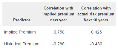
Professor Damodaran is one of the leading proponents of using an implied approach to estimate the Equity Risk Premium. He tested the correlations between his implied Equity Risk Premium methodology and several other approaches, including the historical approach of Ibbotson. Below in Table 1 are the correlations he calculated for the implied and historical Equity Risk Premiums. While neither of the correlations in the right hand column below suggest a strong link between the projected Equity Risk Premium and the Equity Risk Premium actually realized over the following 10 years, it’s noteworthy that the correlation using the historical approach is actually negative!

Table 1: Correlations Between Expected Return and Actual Equity Risk Premiums[2]

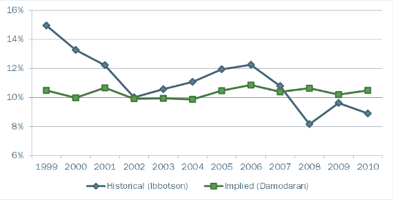
Figure 1 below shows the historical Projected Equity Returns for the period 1999-2010 as calculated using the Ibbotson historical approach and the Damodaran implied approach.

Figure 1: Projected Equity Returns; 1999-2010

Note that the Ibbotson projected equity return moved counter to what might be expected following the crash of 2008, when the projected equity return was lower than at the end of 2007 (8.16% vs. 10.78%). On the other hand, the Damodaran projected equity return increased slightly (10.64% vs. 10.39%). The same holds true for the downturn in 2000-2002. The Ibbotson projected equity return was 14.95% at the end of 1999 and declined to 10.01% at the end of 2002. The projected equity return from Damodaran declined during that same time period, but only from 10.49% to 9.91%. Interestingly, by using an implied Equity Risk Premium, the projected equity return is more stable than under the Ibbotson approach of strictly relying on history.

In 2010, the Delaware Chancery Court issued an opinion in which it ruled in favor of an Equity Risk Premium lower than that produced by Ibbotson’s historical approach. The Chancery Court found in favor of an Equity Risk Premium more in line with one produced by Damodaran’s implied Equity Risk Premium approach.[3] For the reasons stated above, we utilize the implied Equity Risk Premiums as available on Aswath Damodaran’s website. The Equity Risk Premium for the U.S. market as of December 31, 2013 was 4.96%.

Foreign equities are generally considered to be riskier than those in the U.S., with some exceptions for countries such as Switzerland in which typically only the very largest companies are listed on the market and the country itself is stable. In his 2012 book, Investment Valuation, 3rd Edition, Aswath Damodaran provides several alternatives to adjust for the differences in risk from the U.S. market, including adjustments based either on the credit default spreads or the ratings which S&P and Moody’s give the countries’ government securities. We use the ratings from S&P and Moody’s to adjust for differences in country risk.

As of December 31, 2013, the weighted average Equity Risk Premium for the 21 countries comprising the EAFE index was 5.58%, and the weighted average Equity Risk Premium for the emerging markets of Brazil, Russia, India, and China was 6.15%. Stated another way, based on the implied Equity Risk Premium as of December 31, 2013, an investment in a broadly diversified portfolio of stocks within the non-U.S. developed countries should yield an annualized return 62 basis points (5.58%-4.96%) more than a similar investment in U.S. stocks. Likewise, an investment in a broadly diversified portfolio of stocks within the emerging markets should yield an annualized return 119 basis points (6.15%-4.96%) more than a similar investment in U.S. stocks.

D. Size and Value Factor Tilts

Damodaran’s implied Equity Risk Premium is for the broad market, not a portfolio tilted to one or more factors such as smallness and value. Fama/French research, as well as that of others, supports the idea that, over time, smaller stocks outperform larger stocks and high book-to-market stocks outperform low book-to-market stocks. Their research for the period July, 1926-December, 2013 indicates that the additional geometric return for the “smallness” factor is 2.22%/year and for the “value” factor is 4.11%/year. These additional returns are not additive. That is, a portfolio skewed to small value stocks is not expected over time to produce annualized returns 6.33% (2.22% + 4.11%) higher than the broad market. Further, our portfolios don’t, and aren’t intended, to fully capture the incremental return from either of these factors as the additional risk related to doing so becomes significant.

Based on our analysis, an index tilted to “smallness,” such as the Russell 2000 Index, might earn a return over time of 75 basis points more per year than the broad domestic equity market. Similarly, an index tilted to “value,” such as the Russell 1000 Value Index, might earn a return over time of approximately 130 basis points more per year than the broad domestic equity market. We added these incremental expected return premiums to Damodaran’s implied Equity Risk Premiums for funds tilted to size or value based on their market capitalization and price-to-book characteristics.

III. Fixed Income Returns

Studies have shown that the current yield on a 10-year fixed income security is the best predictor of the actual return earned over the ensuing 10 years. According to John Bogle of Vanguard, the current yield on a 10-year Treasury accounts for 92% of the actual return earned over the next 10 years.[4] In our projection of 10-year portfolio returns, we assume that the current yield on the 10-year Treasury equals the return earned on Treasuries over the next 10 years. Utilizing the current yield curve, we make adjustments for securities with shorter or longer durations. For non-Treasury securities, we also adjust for the credit risk using the current spread in yields between comparable duration Treasuries and Corporates.

IV. Geometric vs. Arithmetic Returns

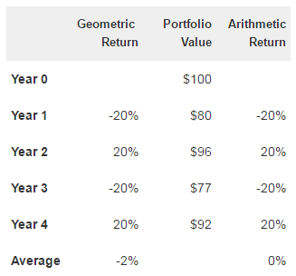
The example below illustrates the difference between the geometric and arithmetic return. Our clients ultimately care about the annualized return they earn over time, which is the geometric return. In the example below, over the 4-year period, the portfolio declined from $100 to $92, or 8%. The annualized, or geometric, return was a negative 2%. However, the arithmetic average of the returns over the 4-year period was 0%.

Table 2: Geometric vs. Arithmetic Return Example

In running Monte Carlo simulations, there is some debate in the literature as to whether it is more appropriate to use geometric or arithmetic returns, with the great majority of academicians favoring the use of arithmetic returns. To test this, we ran multiple instances of a 100,000 scenario, 30-year projection. In each instance, we input the arithmetic return for the S&P 500 from 1926-2012 and the annual standard deviation for the same period. What one would expect is that on average the scenarios would produce a projected geometric return equal to the actual geometric return of the S&P 500 over the 1926-2012 period. Our results produced a geometric return only slightly higher than the actual historical geometric return, which validates the use of arithmetic returns in running Monte Carlo simulations. The formula for converting geometric returns to arithmetic returns is approximately as follows:

Arithmetic Return = Geometric Return + (Variance/2)

V. Summary

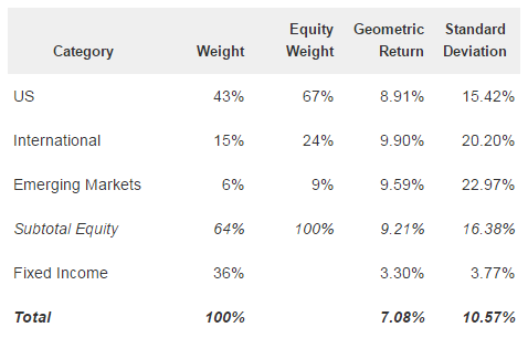
For a diversified portfolio of 64% equities and 36% fixed income, we project as of December 31, 2013, a 10-year annualized portfolio return of 7.1%, with a standard deviation of 10.6%. For the 10-year projection period, our Monte Carlo simulation shows that there is a 52% probability that the investor will achieve a return in excess of 7%. The assumptions underlying this result are shown in Table 3.

Table 3: Projected Portfolio Risk and Return as of December 31, 2013